Exoplanets, and Methods of Detecting Them
In this post I will explain what exoplanets are, how they’re observed, how orbital systems work, and how we can use different techniques - particularly, machine learning - to identify exoplanets in distant star systems.
An exoplanet, or extrasolar planet, is a name referring to planets which orbit stars that aren’t our star. The universe is very big, and the distances between stars are gigantic - so gigantic, we typically can’t directly observe other planets orbiting other stars. It’s even difficult to observe planets within our own solar system, as it took until July 14, 2015 for us to get the first photos of Pluto (which, by the time the New Horizons space probe reached Pluto, wasn’t even classified as a planet anymore!). This means that, in order to determine if exoplanets exist, we have to use different methods to observe them. Unfortunately most exoplanets have negligible mass and size compared to the stars they orbit, and thus they are very very difficult to observe even with extremely powerful telescopes.
Astronomers usually use two main methods of detecting exoplanets, although there are others which are planned to be used in future launches. The first technique is the Doppler method, where one measures the wobble in a star’s orbit due to the gravitational pull of orbiting planets. A planet and star will orbit about their common center of mass, which causes the star to appear to wobble a bit.
This wobbling produces a period redshift and blueshift in the star’s spectrum lines. We measure this quantity along the line of sight at which we observe the system. What we measure in practice is the radial velocity, which is the observed change in the star’s velocity along the line of sight due to the orbiting planet:
\[v_r(t) = K \cos(\omega t + \phi)\]Where: \(v_r(t)\): radial velocity at time \(t\)
\(K\): velocity semi-amplitude (maximum radial velocity shift)
\(\omega\): angular frequency of the orbit = \(\frac{2\pi}{P}\), where \(P\) is the orbital period
\(\phi\): phase angle (depends on where the planet started)
The velocity semi-amplitude is given by:
\[K = \left( \frac{2\pi G}{P} \right)^{1/3} \frac{M_p \sin i}{(M_\star + M_p)^{2/3}} \frac{1}{\sqrt{1 - e^2}}\]Where:
\(G\): gravitational constant
\(M_p\): mass of the planet
\(M_\star\): mass of the star
\(i\): inclination of the orbit to the line of sight (if \(i = 90^\circ\), we’re viewing edge-on)
\(e\): orbital eccentricity
For small planets \(M_p \ll M_\star\), the equation simplifies by dropping \(M_p\) in the denominator. So first, an astronomer will observe the periodic Doppler shift in the spectral lines of a star. Then, they fit the observed change \(v_r(t)\) to extract the orbital parameters of the star. Finally, they infer the minimum mass of the planet, \(M_p \sin i\). The inclination \(i\) is usually unknown unless we combine other methods to solve for this quantity, such as with transits. The issue with this method is that it works best for massive planets that are close to their stars rather than small planets or planets further away from their stars, and we cannot detect planets which have face-on orbits where the inclination \(i\) is zero.
The second method commonly used and the one I use in the project is the transit method. When a planet passes in front of the star, it blocks a fraction of the starlight periodically. By monitoring the star’s light curve, we can detect the presence of a planet, as well as its size, orbital period, and sometimes even its atmospheric composition. We refer to the fraction of the amount of starlight blocked as the transit depth, and denote it as \delta, which we defined as:
\[\delta = \left( \frac{R_p}{R_\star} \right)^2\]Where:
\(R_p\): radius of the planet
\(R_\star\): radius of the star
\(\delta\): proportional drop in light intensity
We refer to the time between transits as the orbital period, denoted as P. Once we find the period, we can calculate the semi-major axis a of the planet’s orbit using the following equation:
\[a^3 = \frac{G M_\star P^2}{4\pi^2} \quad \Rightarrow \quad a = \left( \frac{G M_\star P^2}{4\pi^2} \right)^{1/3}\]\(a\): orbital radius
\(G\): gravitational constant
\(M_\star\): mass of the star
\(P\): orbital period
For circular orbits and central transits, the duration T is approximated by:
\[T \approx \frac{P R_\star}{\pi a}\]From these equations we can infer the radius of the planet, the orbital period of the planet, the orbital distance of the planet, and again, we can even infer the atmospheric features of the planet. The transit method is often used with the Doppler method to identify planets and certain features of these planets. A famous example of the success of this method was the identification of the planet HD 209458 b, nicknamed Osiris. It was the first exoplanet discovered transiting a star and the first one detected with an atmosphere.
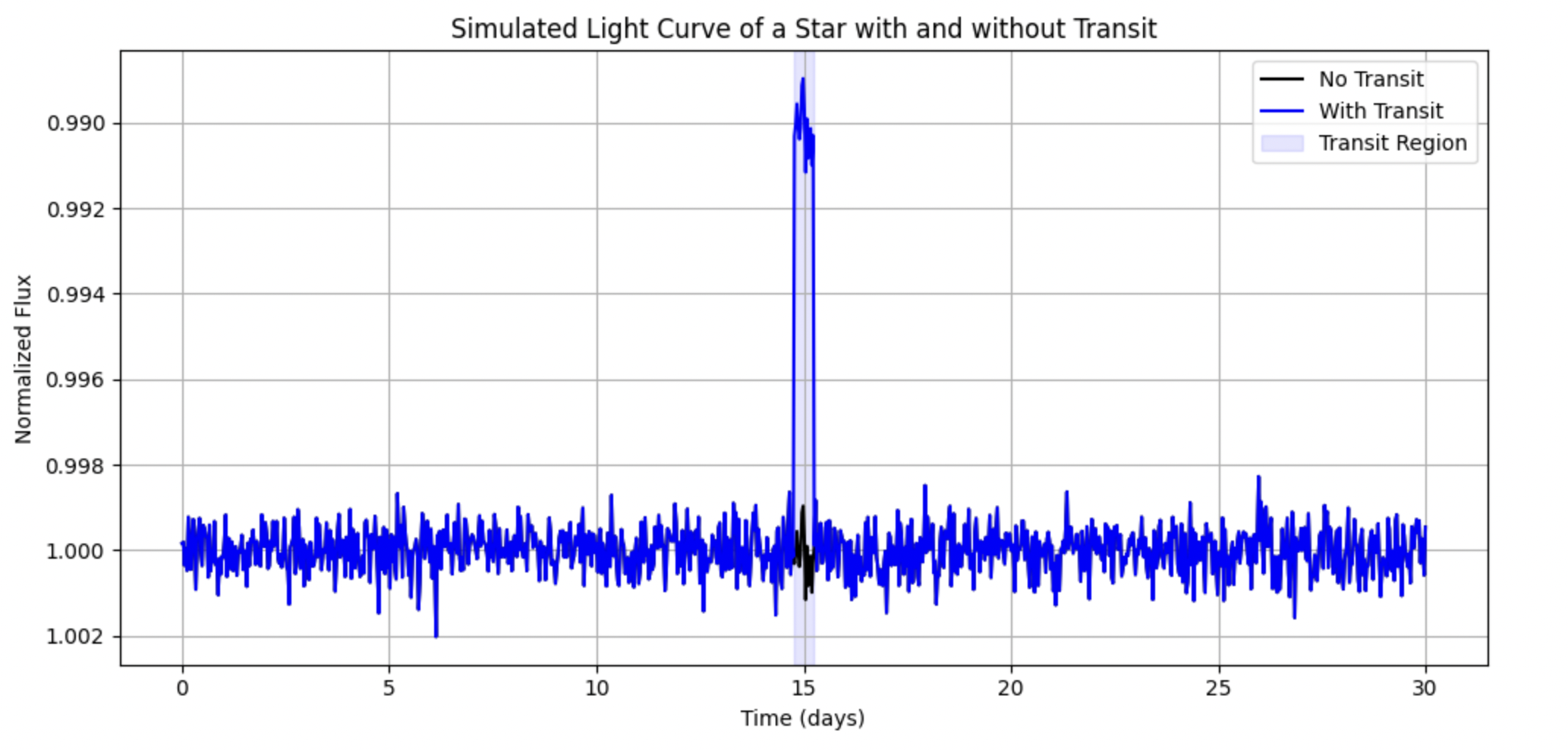
Osiris orbits the star HD 209458 (exoplanets are named by the star they orbit and order of their discovery, so the “b” means it was the first planet discovered orbiting this star), which is a star similar to our Sun but 150 light years away. It is considered a Hot Jupiter type planet, which means it’s a gas giant that orbits very close to its star, making it “hot”. It should also be noted that exoplanet discovery was heavily biased towards these types of stars, as intuitively, it is much easier to discover a large planet that orbits close to its star than a small planet whose orbit would likely take years to come into view, if ever. Its transit was discovered in 1999, and it was discovered to have an atmosphere composed of sodium, hydrogen, water vapor, carbon monoxide, and methane through spectroscopic observations. If we were observing this planet, we would expect to see a lightcurve like this:
| Time (days) | Relative Brightness |
|---|---|
| 0.0 | 1.000 |
| 0.5 | 0.998 |
| 1.0 | 0.985 |
| 1.5 | 0.998 |
| 2.0 | 1.000 |
Where the brightness of the star with no planets in front of it is 1.000, and the brightness at the center of the transit would be 0.985. This table shows a transit dip of 1.5%, which is what we would expect for a large planet passing in front of a star. For spectrum data, we might expect to see something like this telling us what percent of light is getting emitted at what wavelengths after subtracting the stellar spectrum during transit from the one outside of transit:
| Wavelength (nm) | Relative Absorption (%) | Molecule |
|---|---|---|
| 589 | 0.15 | \(Na\) |
| 656 | 0.10 | \(H \alpha\) |
| 940 | 0.25 | \(H_{2}O\) |
| 2300 | 0.30 | \(CO\) |
| 3300 | 0.20 | \(CH_{4}\) |
There are more details that go into this than what I’ve described. For instance, since this is such a sensitive process, we would want to use a space-based telescope to avoid any atmospheric inference. We would have to observe multiple transits to make sure we’re not just seeing space dust or anything else in the interstellar medium that appears like a planet. We would need to have a very good recording of the light curve, so we’re not accidentally misidentifying solar spots or flares as our planet. Fortunately, a lot of data is generated through this process, which means we can apply nifty data analysis tricks to aid in exoplanet identification.
There are multiple transit detection algorithms, but I’ll focus on two for my benchmarking analysis. The first is the box least squares method (BLS), which finds the periodic dips in a light curve caused by a planet moving in front of a star by assuming that the transit signal looks like a box. That means that we are expecting there to be a flat baseline amount of light emitted by the star, then a dip from the planet passing by, and then the flat baseline again. First, we pick a trial period, say two days, where we are observing the transit of the star. Then we align all data points in the light curve to modulo two days, the period. We then fit a box to the folded light curve, and then we check to see how well the box explains the data by seeing how well it minimizes residuals between the data and the model. We quantify the fit with a score we call the power. We do this for thousands of trial periods and durations, and choose the one with the highest power.
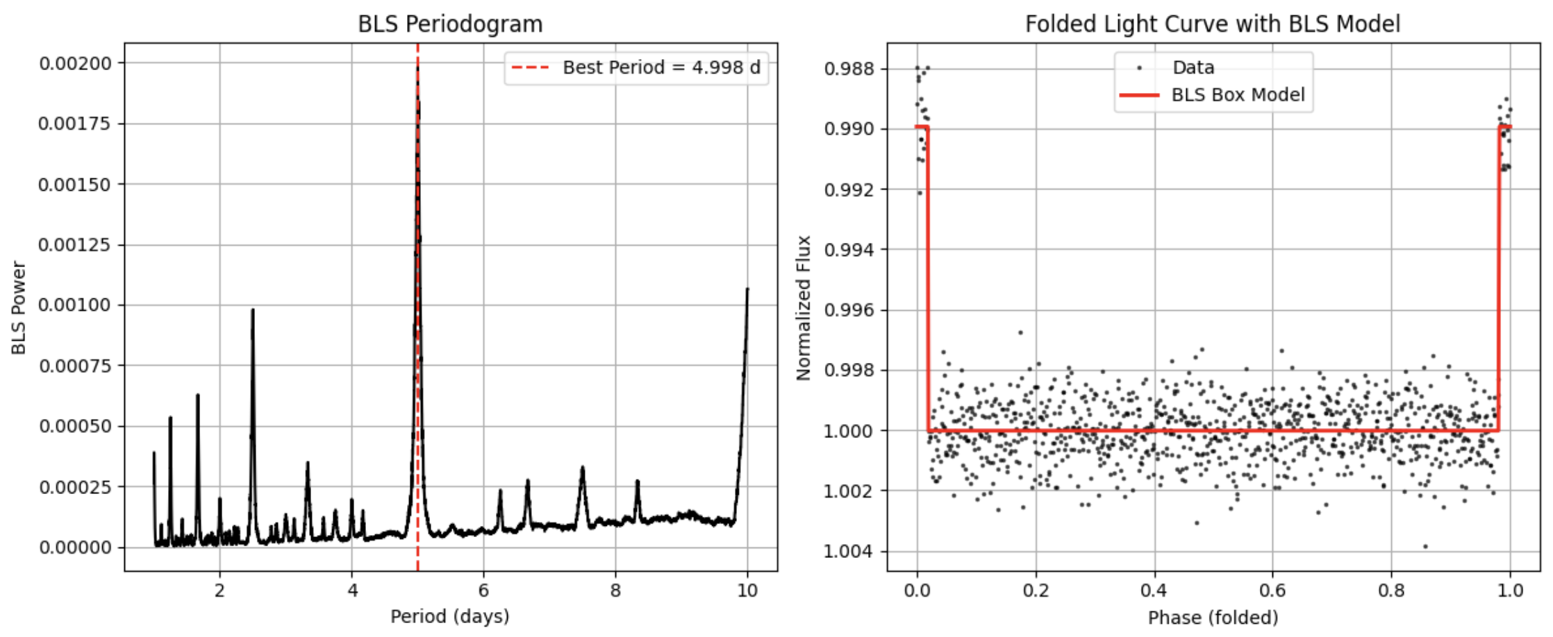
Then, for each period the algorithm will fold the light curve - meaning that the data points are aligned with the period - to a box model, and compute a power to indicate how strong the signal is. With BLS we are sliding a box-shaped model over the data, where a height of one indicates we are out of a transit and a lower depth inside a transit. The box location is at the T0 of the trial. Power is a measure of how box-shaped the transit signal is for the data within a given trial period. The equation for it is:
\[\text{Power} = \frac{\delta^2 \cdot N_{\text{transit}}}{\sigma^2}\]Where:
\(\delta\) = estimated transit depth.
\(N_{\text{transit}}\) = number of in-transit data points.
\(\sigma^{2}\) = variance of the flux.
This is proportional to the signal to noise ratio squared, so higher values mean a stronger detection. BLS works well on big datasets, and since it comes with few assumptions on the underlying data it’s good for periodic dips. However, its one major assumption - that the transit will follow a box shape - is flawed, as planetary transits will have rounded bottoms due to limb darkening. Limb darkening is where the edges of the star look dimmer than the center of the star. The center of the star, when looked on straight ahead, lets you see deeper into the star, where it’s hotter and brighter. But at the edges, you see the cooler upper layers, which emit less light. When the planet passes in front of the star, it blocks less light when crossing the dim edges and blocks more light when it passes over the bright center of the star, which causes the transit curve to be rounded instead of a box.
To fix this issue, transit least squares (TLS) was developed. TLS takes into account limb darkening, stellar noise, and a realistic transit shape, using a matched filter to aid in evaluating the SNR for candidate signals. It has a higher sensitivity, fewer false positives, and a better recovery for smaller planets, but is slower than BLS and more computationally intensive. To perform TLS, we do the same things we did with BLS, but instead of fitting a box we want to fit a realistic transit model. We use physical parameters, such as the planet-to-star ratio, and include limb darkening by assessing the gradual brightness change from the center to the edge of the star. Then, we calculate a signal detection efficiency score for each fit, which measures how likely it is that we have a real transit signal. Finally, we return the best fit parameters for the period, duration, T0 (midpoint of the transit), depth, and SNR to determine the best fit curve.
In this project, I use BLS and TLS as benchmarks first to test my simulation, before attempting to apply machine learning techniques. Before discussing exoplanets and techniques to search for them further, it would be good to discuss how I simulate planetary systems in Python. The equations governing gravitational forces are well-understood and have been well defined for centuries through Newton’s laws of gravitation. The gravitational force between two bodies i and j is computed using the following equation:
\[F = G \frac{m_i m_j}{r_{ij}^2}\]Where:
\(G\) is the gravitational constant (possibly normalized)
\(r_{ij}\) is the distance between the two bodies
Each body experiences the net force from all other bodies, requiring an \(\mathcal{O}(N^2)\) loop over all body pairs. We can solve for the velocity and position with the following equations:
\[\vec{v}_{t+\Delta t} = \vec{v}_t + \vec{a}_t \Delta t\] \[\vec{x}_{t+\Delta t} = \vec{x}_t + \vec{v}_{t+\Delta t} \Delta t\]To build the simulation in Python, we will expand these equations using numerical methods. In simulation.py I implement three integration methods for this purpose: Euler step, velocity verlet step, and RK4, which I discussed in my Lorenz system post. The Euler step simply computes the values per time step, and the velocity verlet step computes the one-half time step as in the following equations:
\[\vec{v}_{t+\frac{1}{2}} = \vec{v}_t + \frac{1}{2} \vec{a}_t \Delta t\] \[\vec{x}_{t+1} = \vec{x}_t + \vec{v}_{t+\frac{1}{2}} \Delta t\] \[\vec{v}_{t+1} = \vec{v}_{t+\frac{1}{2}} + \frac{1}{2} \vec{a}_{t+1} \Delta t\]
Real systems are three dimensional, and thus also have the other dimensions of inclination and eccentricity. The inclination \(i\) is the tilt of the planet’s orbit’s plane relative to a reference plane. For an inclination between zero and ninety degrees, we call this a prograde orbit; for ninety degrees, a polar orbit; and for greater than ninety degrees, a retrograde orbit. Eccentricity \(e\) is a measure of how far the orbit is from being a perfect circle. It is measured as the square root of one minus the ratio of the squares of the semi-minor axis to the semi-major axis of the ellipse. For an eccentricity of zero, we have a perfect circle; for between zero and one, we have an ellipse; and for greater than one, we have a hyperbola, or an unbound orbit.

It is now simple enough to compute the 3D visualization for the moving planets with eccentricities and inclinations accounted for, using Kepler’s equation to solve for where along the ellipse the object current is and saving the vector path for the planet along its orbit. Below is an animation showing this 3D model of a star system:
Now, we can generate simulated data like that captured from major exoplanet search satellites. There are several satellites which have discovered or are planned to discover exoplanets. The most famous and most prominent is the Kepler Space Telescope, active from 2009-2018. This venerable mission was aimed at measuring the frequency of Earth-like planets in the habitable zone around stars. Using the transit method, it discovered around 2700 exoplanets in the Cygnus-Lyra region. After Kepler was TESS, or the Transiting Exoplanet Survey Satellite, launched in 2018 and still active today. Its mission was to survey the entire sky, but especially focused on closer and brighter stars, which would make spectroscopic follow-up easier. Then there is CHEOPS, or CHaracterising ExOPlanet Satellite, launched by the ESA (European Space Agency) in 2019 and still currently active. And finally, there is the Roman Space Telescope, which is planned to be launched in 2027. This one would use microlensing to discover new planets and present an exciting avenue for future searches. There are a few others which don’t necessarily use the transit method as much and don’t have the same mission of only detecting exoplanets, instead using exciting methods like astrometry, infrared imaging, or even asteroseismology, but I won’t examine them for the purposes outlined here.
In the next post, I will explain various machine learning models I try to approach this problem with, such as convolutional neural networks, Bayesian neural nets, and other approaches that can 1) aid in exoplanet detection, but also 2) improve the interpretability of machine learning methods applied to these datasets and 3) be used in different systems such as unstable systems or eclipsing binaries to aid with these and future searches.