Developing a Lorenz Attractor in Assembly
In this post I aim to outline and explain the Lorenz attractor, and show how I can build a simulation for the attractor in the Assembly programming language.
The Lorenz attractor is a set of chaotic solutions to the following system of three differential equations:
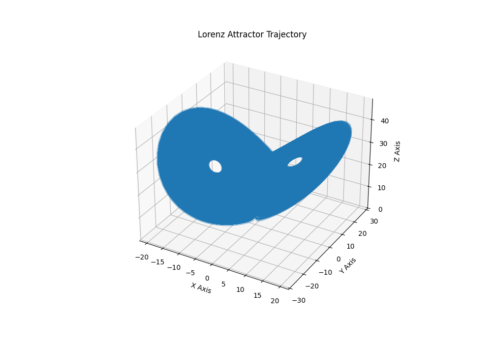
\[\frac{dx}{dt} = \sigma (y - x)\] \[\frac{dy}{dt} = x(\rho - z) - y\] \[\frac{dz}{dt} = xy - \beta z\]Edward Lorenz, after whom this solution is named, formalized the Lorenz attractor in 1963 while studying atmospheric convection. This system follows well-defined rules but behaves unpredictably as it evolves, and thus falls into the category of “deterministic chaos”. What’s interesting is that when these equations are solved and plotted on a three dimensional graph, you get a butterfly-shaped structure (this is actually where the term “butterfly effect” comes from). If we consider two neighboring points, we observe that they diverge rapidly from each other, and their divergence is heavily dependent on the initial conditions - however, this motion tends to be relegated to a bounded, fractal-like region, in which the same pattern is observed at smaller and smaller scales.
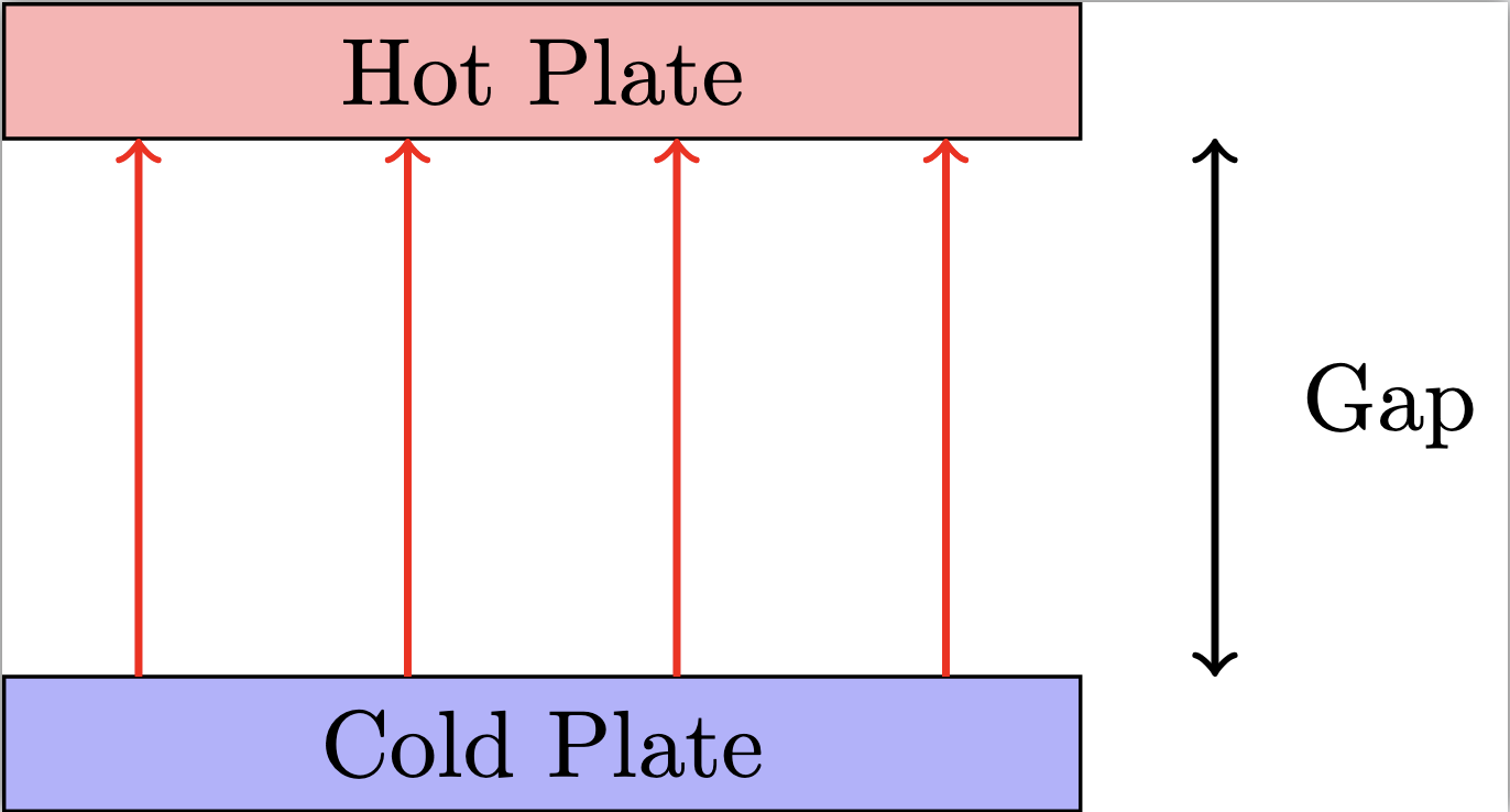
Lorenz approached the problem in the context of atmospheric convection. He was studying how hot air rose, and cool air sank, between two plates of different temperatures in a cycle called Rayleigh-Benard convection. Rayleigh-Benard convection refers to a type of fluid motion in which a fluid is heated from below and cooled from above. The behavior of this fluid is exciting, as rather than simply conducting heat, the fluid will spontaneously start to move, forming convection cells. The motion of air is described by fluid equations - as air is a fluid - and thus one would look at the relevant Navier-Stokes equations, heat equation, and boundary conditions to analyze this system. These formulas result in complicated partial differential equations, and Lorenz preferred simplifying this system to an easier model. In order to simplify this system, some assumptions have to be made.
The system consists of two parallel plates of differing temperatures, so we assume there is 2D flow in the x and z directions (horizontal and vertical). We will also assume periodic and simple boundary conditions. This condition is a bit funny - essentially, we’re assuming that, like in a 2D video game, when you move off-screen to the right you loop back around to the other side, meaning we won’t have to really consider the horizontal boundaries and assume the system is self-contained. We’re also assuming that the plates themselves are just ideal plates with no unexpected (in a mathematical rather than physical sense) behaviors. Finally, we keep only the largest modes of motion, truncating the higher-frequency variations. A mode of motion is a specific pattern of movement for a general object, which is easier to picture when you imagine the ripples in a pond. When we say we’re truncating the higher-frequency variations, we’re looking at the modes of motion of air - the swirling currents created, like on a windy day - and removing the eddies and and tiny ripples so we can see the bigger picture, the convections created by temperature gradients within the fluid.

Having established our simplifying assumptions for the model, we then expand the fluid velocity and temperature fields in terms of Fourier series, keeping only the three most dominant terms: the convection roll intensity, the horizontal temperature variation, and the vertical temperature variation. (Note: cutting only a few modes in a Fourier expansion is called Galerkin truncation.) The fluid velocity is given as:
\[\mathbf{v} = (u(x,z,t), w(x,z,t))\]where:
\(u(x,z,t)\) = horizontal velocity (in x),
\(w(x,z,t)\) = vertical velocity (in z).
However, because Lorenz wanted a simple model, he made an assumption about the incompressibility of the function:
\[\frac{\partial u}{\partial x} + \frac{\partial w}{\partial z} = 0\]And further used a stream function $\psi(x,z,t)$ to satisfy the incompressibility condition:
\[u = \frac{\partial \psi}{\partial z}, \quad w = -\frac{\partial \psi}{\partial x}\]So once you know \(\psi(x,z,t)\), you can compute both \(u\) and \(w\).
The temperature field is given as:
\[T(x,z,t) = B(t) \cos\left(\frac{\pi x}{L}\right) \sin(\pi z) + C(t) \sin(2\pi z)\]where:
\(B(t)\) = amplitude of horizontal temperature variation,
\(C(t)\) = amplitude of vertical temperature deviation.
Lorenz expanded the fields into simple trigonometric modes in order to expand the above equations in terms of Fourier series. He proposed the following stream function for the fluid velocity:
\[\psi(x, z, t) = A(t) \sin\left(\pi z\right) \sin\left(\frac{\pi x}{L}\right)\]where:
\(A(t)\) is a time-dependent amplitude, \(L\) is the aspect ratio of the domain.
From this we can define the horizontal velocity as:
\[u(x,z,t) = \frac{\partial \psi}{\partial z} = A(t) \pi \cos(\pi z) \sin\left(\frac{\pi x}{L}\right)\]And the vertical velocity as:
\[w(x,z,t) = -\frac{\partial \psi}{\partial x} = -A(t) \frac{\pi}{L} \sin(\pi z) \cos\left(\frac{\pi x}{L}\right)\]But remember, only a few modes were kept, those being the lowest-frequency, or largest scale, patterns in the oscillations of the field. The convection mode captures the rise and fall of the fluid; the horizontal temperature mode captures how the temperature gradient develops; and the vertical temperature mode captures how the temperature’s vertical profile is nonlinear, describing the bulges in the temperature front.
Next, we define a few variables to build our system of equations. First, we define \(x(t)\), the intensity of the convection rolls; \(y(t)\), the temperature difference across the rolls and horizontal temperature variation; and \(z(t)\), the vertical temperature deviation from linear. We refer to these as the amplitudes of the main modes of motion. We then substitute the Fourier series into the full fluid equations to get the following three ordinary differential equations:
\[\frac{dx}{dt} = \sigma (y - x)\]Where sigma is the Prandtl number, measuring the ratio of fluid viscosity to thermal diffusivity,
\[\frac{dy}{dt} = x (\rho - z) - y\]Where rho is the Rayleigh number, measuring how strong the temperature gradient is across the plates, and
\[\frac{dz}{dt} = xy - \beta z\]Where beta is the geometry of the convection rolls.
These equations are nonlinear, as the variables are coupled together, allowing energy to move around randomly throughout the system. Small changes in the initial values cause the system to have exponentially amplified differences over time, and the system has feedback loops that amplifies the chaos of the system. What we see here is that, from a simple system (although with a somewhat complicated mathematical description), emerges well-described chaos.
So, to sum, the Lorenz system is deterministic - knowing the initial conditions means we can absolutely determine the future conditions. Yet the system is extremely sensitive to its initial conditions, so much so that we need to very very very precisely know the initial conditions if we want to determine future conditions, and any small deviation will cause significantly different results. However, despite this, the system stays bounded, so it does not blow up to infinity over time, and it does not settle to one point but instead swirls around in a pattern termed the attractor. This, at its heart, is what chaos is - predictability in a system has a time limit after which we can no longer predict the long-term outcome of a system.
We can analyze the behavior of the Lorenz attractor ourselves by building it in the Assembly programming language. Assembly allows us to meticulously build every numerical step in low-level instructions directly fed to the computer, giving us direct control over implementing the system and creating an extremely fast simulation. The benefit of building a simulation is that it’s cool - I get to see a diagram and feel the satisfaction of realizing the equations. Additionally, I then get to build off of that simulation, and extend the problem to other questions. I can build the foundations for a toolbox of sorts, allowing me to quickly develop new models based off of the model I already built. Finally, it allows me to implement exciting computational methods in order to solve this problem in a way a machine would understand, saddling between the mathematical and computational side of the problem. The Lorenz attractor is already a well-understood and well-analyzed system of equations, which could be easily implemented in higher-level languages. However, by using Assembly, I hope to get finer control over the steps of computation so I can better analyze the system. For one, I prefer being able to control the addition, subtraction, multiplication, memory load, and store operations, so I can see how chaotic behavior is built directly from primitive numerical steps. Also, Assembly is notoriously fast, which is an exciting thing to see in action.
I’ve written an implementation of the Lorenz system in x86-64 assembly (you can find the full Assembly code here on GitHub), using the Runge-Kutta 4th order method (RK4) to numerically integrate the differential equations. RK4 is a numerical algorithm (a method for solving an equation step-by-step with numbers instead of symbols) for solving ordinary differential equations. It samples the slopes of the data at several intermediate points to give us higher precision, which is ideal for solving a chaotic system where the behavior can be unpredictable. For a general system:
\[\frac{dy}{dt} = f(y, t)\]The RK4 update rule is:
\[k_1 = f(y_n, t_n)\] \[k_2 = f\left(y_n + \frac{h}{2}k_1, t_n + \frac{h}{2}\right)\] \[k_3 = f\left(y_n + \frac{h}{2}k_2, t_n + \frac{h}{2}\right)\] \[k_4 = f\left(y_n + hk_3, t_n + h\right)\]So then we can solve for the next value:
\[y_{n+1} = y_n + \frac{h}{6}(k_1 + 2k_2 + 2k_3 + k_4)\]where h is the time step. Essentially, RK4 uses a weighted average of the slopes to solve for the next value. The Lorenz attractor uses three coupled ODEs described above, so we have to apply RK4 separately to each variable x, y, and z.
Assembly is machine code, communicating directly with the machine. There are no variables or functions, and we have to manage the memory and calculation steps directly ourselves. It is a bit of a headache having to manually control every element of the routine, especially for someone like me coming from a Python-heavy background where these things are not only taken for granted but not even considered. As a broad overview of what’s going on in the code, first I initialize x=0, y=1, and z=1 and load the total number of steps, 10000, into the register ecx. Then, in the main loop, .loop, I save the original state x, y, and z to variables orig_x, orig_y, and orig_z. I compute k1 for each variable in derivatives for the initial point and store those values in their corresponding variables. Then, I restore the original state again, update them with midpoint_update, call derivates again, and compute k2. Doing this for k3 and k4, I then computer the RK4 step with the formula:
\[x_{\text{new}} = x_{\text{old}} + \frac{h}{6}(k_1 + 2k_2 + 2k_3 + k_4)\]I use printf to return the values of x, y, and z after the update, and then decrement ecx. I check if ecx is zero, and if not, loop through the whole function again to get the next update in the steps. This builds my Lorenz attractor in three dimensions, the plot of which is shown below.